import matplotlib.pyplot as plt
import numpy as np
All vectors in the vector space has a length except \(0\)-vector, and the terminology of length is norm, the general formula of norm of a vector in \(\mathbb{R}^k\) is given by
\[ \|u\|= \sqrt{x_1^2+x_2^2+...+x_k^2} \]
As an example, let’s plot vectors \((4, 7)\) and \((8, 6)\) in \(\mathbb{R}^2\).
# Define the figure and axis
fig, ax = plt.subplots(figsize=(8, 8))

# Define the vectors as starting points and directions
vectors = np.array([[0, 0, 4, 7], [0, 0, 8, 6]])

# Unpack the vectors into separate components
X, Y, U, V = zip(*vectors)

# Plot the vectors using quiver
ax.quiver(X, Y, U, V, angles="xy", scale_units="xy", scale=1, color="red", alpha=0.6)

# Set the limits and labels for the plot
ax.set_xlim([0, 10])
ax.set_ylim([0, 10])
ax.set_xlabel("x-axis", fontsize=16)
ax.set_ylabel("y-axis", fontsize=16)

# Add grid
ax.grid()

# Annotate the end points of the vectors
ax.text(4, 7, "$(4, 7)$", fontsize=16)
ax.text(8, 6, "$(8, 6)$", fontsize=16)

# Draw lines to the origin for the first vector
ax.plot([4, 4], [0, 7], color="blue", linewidth=2)
ax.plot([0, 4], [0, 0], color="blue", linewidth=2)

# Draw lines to the origin for the second vector
ax.plot([8, 0], [0, 0], color="blue", linewidth=2)
ax.plot([8, 8], [0, 6], color="blue", linewidth=2)

# Annotate the magnitudes of the vectors using Pythagorean theorem
ax.text(
    1.7, 3.8, r"$\sqrt{4^2+7^2}$", fontsize=16, rotation=np.arctan(7 / 4) * 180 / np.pi
)
ax.text(
    5, 4.1, r"$\sqrt{8^2+6^2}$", fontsize=16, rotation=np.arctan(6 / 8) * 180 / np.pi
)

# Show the plot
plt.show()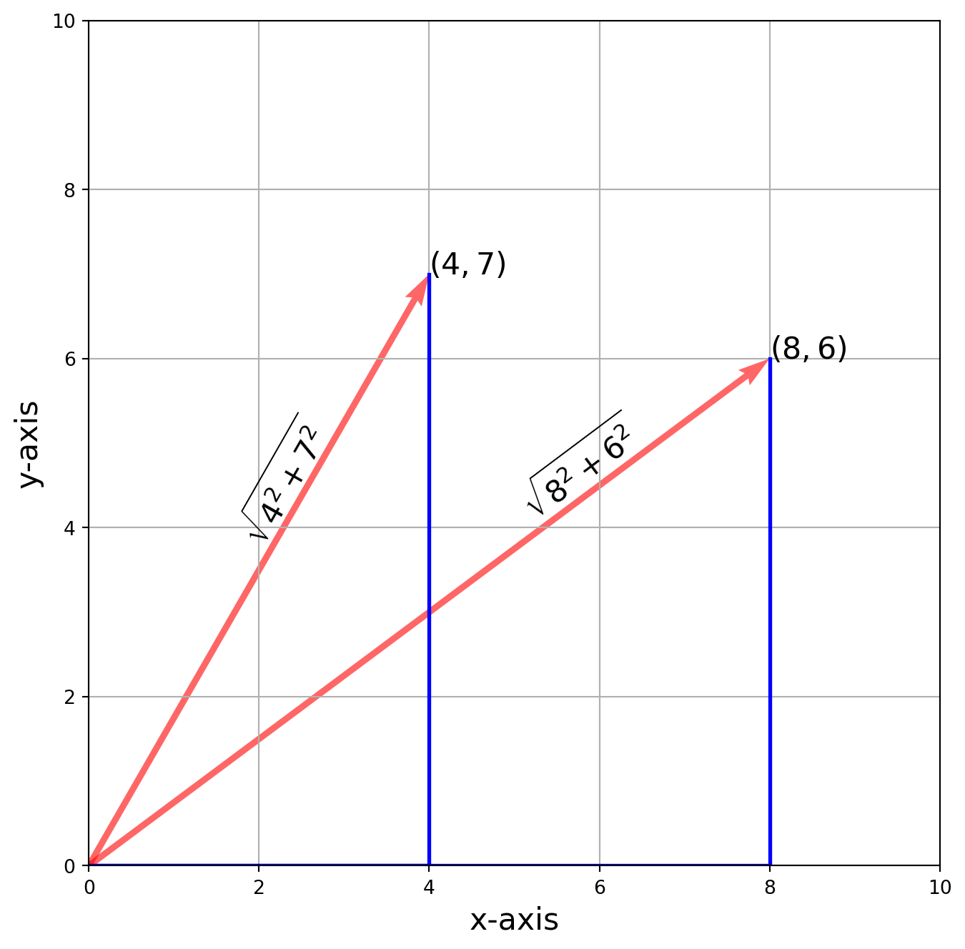
There is also a NumPy function for computing norms: np.linalg.norm().
a = np.array([4, 7])
b = np.array([8, 6])
a_norm = np.linalg.norm(a)
b_norm = np.linalg.norm(b)
print("Norm of a and b are {0:.4f}, {1} respectively.".format(a_norm, b_norm))
Norm of a and b are 8.0623, 10.0 respectively.Let’s try plotting vectors \((1, 1, 1)\), \((-2, 2, 5)\), \((3, -2, 1)\) in \(\mathbb{R}^3\).
fig = plt.figure(figsize=(10, 10))
ax = fig.add_subplot(111, projection="3d")

vec = np.array([[0, 0, 0, 1, 1, 1], [0, 0, 0, -2, 2, 5], [0, 0, 0, 3, -2, 1]])
X, Y, Z, U, V, W = zip(*vec)
ax.quiver(
    X,
    Y,
    Z,
    U,
    V,
    W,
    length=1,
    normalize=False,
    color="red",
    alpha=0.6,
    arrow_length_ratio=0.18,
    pivot="tail",
    linestyles="solid",
    linewidths=3,
)

ax.set_xlim([-5, 5])
ax.set_ylim([-5, 5])
ax.set_zlim([0, 5])

ax.text(1, 1, 1, "$(1, 1, 1)$")
ax.text(-2, 2, 5, "$(-2, 2, 5)$")
ax.text(3, -2, 1, "$(3, -2, 1)$")
ax.text(0, 0, 0, "$(0, 0, 0)$")

points = np.array(
    [
        [[1, 1, 1], [1, 1, 0]],
        [[0, 0, 0], [1, 1, 0]],
        [[3, -2, 1], [3, -2, 0]],
        [[0, 0, 0], [3, -2, 0]],
        [[-2, 2, 5], [-2, 2, 0]],
        [[0, 0, 0], [-2, 2, 0]],
    ]
)

for i in range(points.shape[0]):  # loop through the 3rd axis
    X, Y, Z = zip(*points[i, :, :])
    ax.plot(X, Y, Z, lw=2, color="b", alpha=0.7)
ax.grid()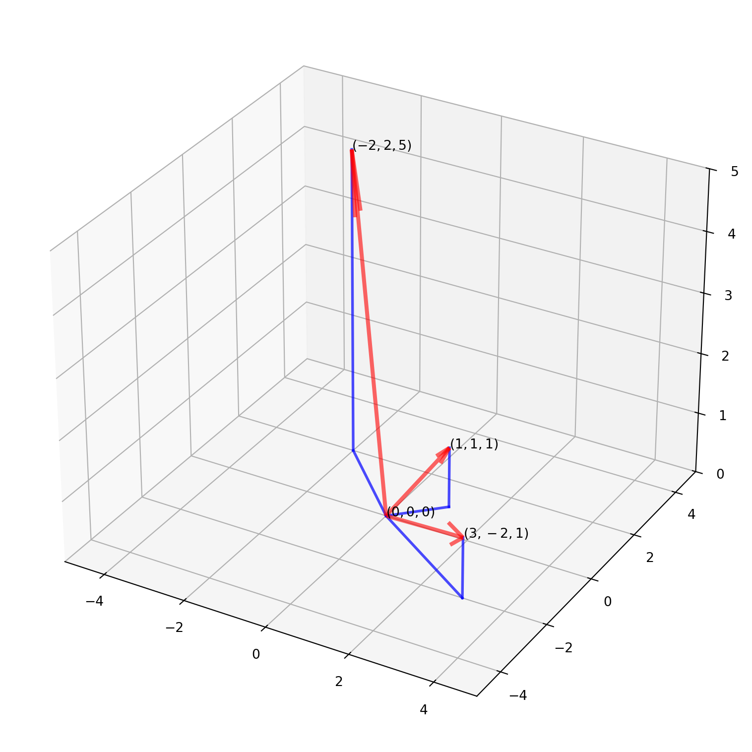
So the norm of vectors are quite obvious once you see their coordinates.
Vector Addition, Subtraction And Scalar Multiplication
The vector addition is element-wise operation, if we have vectors \(\mathbf{u}\) and \(\mathbf{v}\) addition:
\[\mathbf{u}+\mathbf{v}=\left[\begin{array}{c} u_{1} \\ u_{2} \\ \vdots \\ u_{n} \end{array}\right]+\left[\begin{array}{c} v_{1} \\ v_{2} \\ \vdots \\ v_{n} \end{array}\right]=\left[\begin{array}{c} u_{1}+v_{1} \\ u_{2}+v_{2} \\ \vdots \\ u_{n}+v_{n} \end{array}\right]\]
And subtraction: \[\mathbf{u}+(-\mathbf{v})=\left[\begin{array}{c} u_{1} \\ u_{2} \\ \vdots \\ u_{n} \end{array}\right]+\left[\begin{array}{c} -v_{1} \\ -v_{2} \\ \vdots \\ -v_{n} \end{array}\right]=\left[\begin{array}{c} u_{1}-v_{1} \\ u_{2}-v_{2} \\ \vdots \\ u_{n}-v_{n} \end{array}\right]\]
And the scalar operations: \[c \mathbf{u}=c\left[\begin{array}{c} u_{1} \\ u_{2} \\ \vdots \\ u_{n} \end{array}\right]=\left[\begin{array}{c} c u_{1} \\ c u_{2} \\ \vdots \\ c u_{n} \end{array}\right]\]
Let’s illustrate vector addition \(\mathbf{u}+\mathbf{v}\) in both \(\mathbb{R}^2\) and \(\mathbb{R}^3\).
fig, ax = plt.subplots(figsize=(9, 9))

vec = np.array(
    [[[0, 0, 4, 7]], [[0, 0, 8, 4]], [[0, 0, 12, 11]], [[4, 7, 8, 4]], [[8, 4, 4, 7]]]
)
color = ["r", "b", "g", "b", "r"]

for i in range(vec.shape[0]):
    X, Y, U, V = zip(*vec[i, :, :])
    ax.quiver(
        X, Y, U, V, angles="xy", scale_units="xy", color=color[i], scale=1, alpha=0.6
    )

ax.set_xlim([0, 15])
ax.set_ylim([0, 15])
ax.set_xlabel("x-axis", fontsize=16)
ax.set_ylabel("y-axis", fontsize=16)
ax.grid()

for i in range(3):
    ax.text(
        x=vec[i, 0, 2],
        y=vec[i, 0, 3],
        s="(%.0d, %.0d)" % (vec[i, 0, 2], vec[i, 0, 3]),
        fontsize=16,
    )

ax.text(x=vec[0, 0, 2] / 2, y=vec[0, 0, 3] / 2, s="$u$", fontsize=16)
ax.text(x=8, y=9, s="$v$", fontsize=16)
ax.text(x=6, y=5.5, s="$u+v$", fontsize=16)

ax.set_title("Vector Addition", size=18)
plt.show()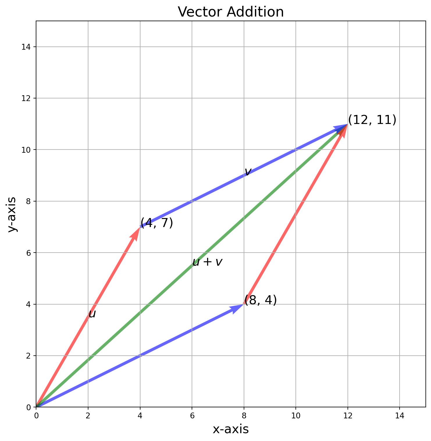
The illustration of \(\mathbf{u} - \mathbf{v}\) is exactly equivalent to \(\mathbf{u} + (-\mathbf{v})\).
fig, ax = plt.subplots(figsize=(9, 9))

vec = np.array(
    [
        [[0, 0, 4, 7]],
        [[0, 0, 8, 4]],
        [[0, 0, -8, -4]],
        [[0, 0, -4, 3]],
        [[-8, -4, 4, 7]],
        [[4, 7, -8, -4]],
        [[8, 4, -4, 3]],
    ]
)
color = ["r", "b", "b", "g", "r", "b", "g"]

for i in range(vec.shape[0]):
    X, Y, U, V = zip(*vec[i, :, :])
    ax.quiver(
        X, Y, U, V, angles="xy", scale_units="xy", color=color[i], scale=1, alpha=0.6
    )

for i in range(4):
    ax.text(
        x=vec[i, 0, 2],
        y=vec[i, 0, 3],
        s="(%.0d, %.0d)" % (vec[i, 0, 2], vec[i, 0, 3]),
        fontsize=16,
    )

s = ["$u$", "$v$", "$-v$", "$u-v$"]
for i in range(4):
    ax.text(x=vec[i, 0, 2] / 2, y=vec[i, 0, 3] / 2, s=s[i], fontsize=16)
ax.text(x=5.8, y=5.8, s="$u-v$", fontsize=16)

ax.set_xlim([-9, 9])
ax.set_ylim([-9, 9])
ax.set_xlabel("x-axis", fontsize=16)
ax.set_ylabel("y-axis", fontsize=16)
ax.grid()
ax.set_title("Vector Subtraction", size=18)
plt.show()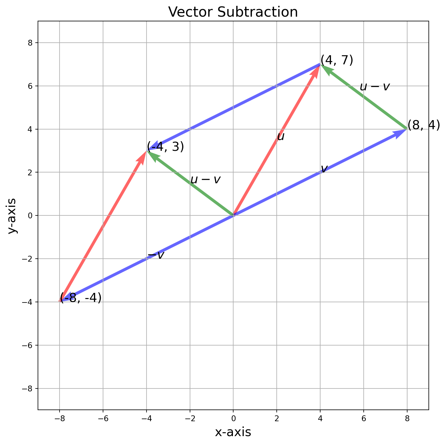
The real number \(c\) in front of vectors are scalars, which are scaling the vectors as its name implies.
fig, ax = plt.subplots(figsize=(9, 9))

vec = np.array([[[0, 0, 2, 3]], [[0, 0, 6, 9]], [[0, 0, 2, 2]], [[0, 0, 8, 8]]])
colors = ["r", "b", "r", "b"]

for i in range(vec.shape[0]):
    X, Y, U, V = zip(*vec[i, :, :])
    ax.quiver(
        X,
        Y,
        U,
        V,
        angles="xy",
        scale_units="xy",
        color=color[i],
        scale=1,
        alpha=0.6,
        zorder=-i,
    )

s = ["$u$", "$3u$", "$v$", "$3v$"]
for i in range(vec.shape[0]):
    ax.text(
        x=vec[i, 0, 2],
        y=vec[i, 0, 3],
        s="(%.0d, %.0d)" % (vec[i, 0, 2], vec[i, 0, 3]),
        fontsize=16,
    )
    ax.text(x=vec[i, 0, 2] / 2, y=vec[i, 0, 3] / 2, s=s[i], fontsize=20)


ax.set_xlim([0, 10])
ax.set_ylim([0, 10])
ax.set_xlabel("x-axis", fontsize=16)
ax.set_ylabel("y-axis", fontsize=16)
ax.grid()

ax.set_title("Vector Multiplication", size=18)
plt.show()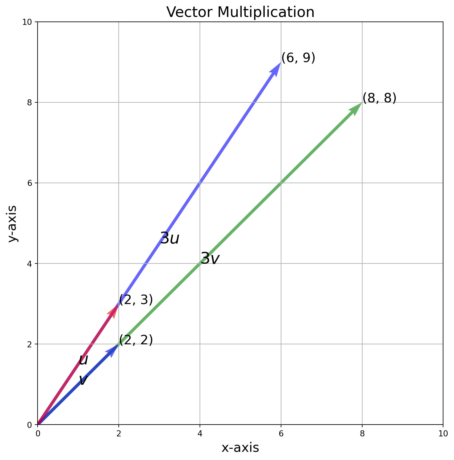
Now let’s challenge ourselves for plotting in 3D.
fig = plt.figure(figsize=(10, 10))
ax = fig.add_subplot(111, projection="3d")

############################## Arrows and Texts #####################################

vec = np.array(
    [
        [[0, 0, 0, 3, 4, 5]],
        [[0, 0, 0, 3, 6, 2]],
        [[0, 0, 0, 6, 10, 7]],
        [[3, 4, 5, 3, 6, 2]],
        [[3, 6, 2, 3, 4, 5]],
        [[0, 0, 0, 8, 2, 2]],
        [[0, 0, 0, 4, 1, 1]],
    ]
)
colors = ["r", "b", "g", "b", "r", "r", "b"]

for i in range(vec.shape[0]):
    X, Y, Z, U, V, W = zip(*vec[i, :, :])
    ax.quiver(
        X,
        Y,
        Z,
        U,
        V,
        W,
        length=1,
        normalize=False,
        color=colors[i],
        alpha=0.6,
        arrow_length_ratio=0.08,
        pivot="tail",
        linestyles="solid",
        linewidths=3,
    )
    ax.text(
        x=vec[i, 0, 3],
        y=vec[i, 0, 4],
        z=vec[i, 0, 5],
        s="$(%.0d, %.0d, %.0d)$" % (vec[i, 0, 3], vec[i, 0, 4], vec[i, 0, 5]),
    )

############################## Axis #####################################
ax.grid()
ax.set_xlim([0, 10])
ax.set_ylim([0, 10])
ax.set_zlim([0, 10])
ax.set_title("Vector Addition and Scalar Multiplication", size=16)
plt.show()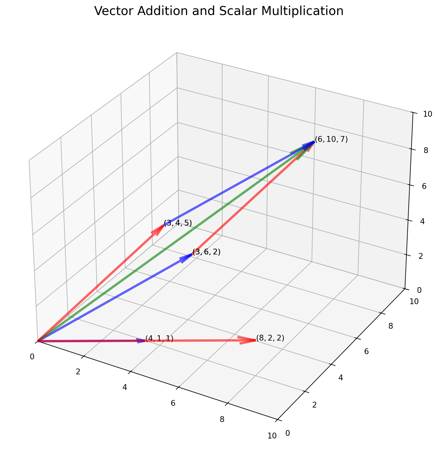
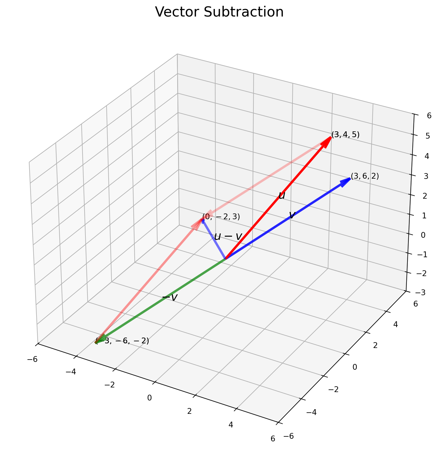
Similarly with \(\mathbf{u}-\mathbf{v}\).
fig = plt.figure(figsize=(10, 10))
ax = fig.add_subplot(111, projection="3d")

############################## Arrows and Texts #####################################

vec = np.array(
    [
        [[0, 0, 0, 3, 4, 5]],
        [[0, 0, 0, 3, 6, 2]],
        [[0, 0, 0, -3, -6, -2]],
        [[0, 0, 0, 0, -2, 3]],
        [[-3, -6, -2, 3, 4, 5]],
        [[3, 4, 5, -3, -6, -2]],
    ]
)
for i in range(vec.shape[0]):
    X, Y, Z, U, V, W = zip(*vec[i, :, :])
    ax.quiver(
        X,
        Y,
        Z,
        U,
        V,
        W,
        length=1,
        normalize=False,
        color=colors[i],
        arrow_length_ratio=0.08,
        pivot="tail",
        linestyles="solid",
        linewidths=3,
        alpha=1 - 0.15 * i,
    )
    ax.text(
        x=vec[i, 0, 3],
        y=vec[i, 0, 4],
        z=vec[i, 0, 5],
        s="$(%.0d, %.0d, %.0d)$" % (vec[i, 0, 3], vec[i, 0, 4], vec[i, 0, 5]),
    )

s = ["$u$", "$v$", "$-v$", "$u-v$"]
for i in range(4):
    ax.text(
        x=vec[i, 0, 3] / 2,
        y=vec[i, 0, 4] / 2,
        z=vec[i, 0, 5] / 2,
        s=s[i],
        size=15,
        zorder=i + vec.shape[0],
    )

############################## Axis #####################################

ax.grid()
ax.set_xlim([-6, 6])
ax.set_ylim([-6, 6])
ax.set_zlim([-3, 6])

ax.set_title("Vector Subtraction", size=18)
plt.show()